Understanding and comparing instrument specifications

Specifications for precision instruments are often complex and difficult to interpret. Users should consider easily overlooked details in order to properly compare these instruments or apply them to their workload.

The initial selection of prospective equipment is usually based on its written specifications. They provide a means for determining the equipment’s suitability for a particular application. Specifications are a written description of the instrument’s performance in quantifiable terms and apply to the population of instruments having the same model number. Since specifications are based on the performance statistics of a sufficiently large sample of instruments, they describe group behavior rather than that for a single, specific instrument.

Good specifications have the following characteristics:

• complete for anticipated applications easy to interpret and use.
• define the effects of environment and loading.

Completeness requires that enough information be provided to permit the user to determine the bounds of performance for all anticipated outputs (or inputs), for all possible environmental conditions within the listed bounds, and for all permissible loads. It is not a trivial task even for a simple standard. Designing complete specifications for a complex instrument like a multifunction or multi-product calibrator is a big challenge.

Ease of use is also important. A large array of specifications, including modifying qualifications and adders, can be confusing and difficult to interpret. Mistakes in interpretations can lead to application errors or faulty calibrations.

The requirement for completeness conflicts somewhat with that for ease of use; one can be traded for the other. The challenge of specification design is to mutually satisfy both requirements.

This is sometimes satisfied by bundling the effects of many error contributions within a window of operation. For example, the listed performance may be valid for six months in a temperature range of 23 ± 5 °C, for rh up to 80 %, for power line voltage of nominal ± 10 %, and for all loads up to the maximum rated current. This is a great simplification for the user since the error contributions of time, temperature, humidity, power line fluctuations and loads can be ignored as long as operation is maintained within the listed bounds.

Since specifications are complex for complex instruments, they can be misused and abused both by users and manufacturers. Reputable manufacturers will attempt to describe the performance of the product as accurately and simply as possible without hiding areas of poor performance by omission of relevant specifications.

Much of the following material describes the effects of incomplete specifications, and how specifications can be misinterpreted or abused.

The various specifications fall into three distinct categories; these will be defined later. Each specification must be carefully considered when comparing instruments from different vendors. All of these components combine to describe the performance of a given instrument. Purchasers need to be proficient at adding the contribution of each component to arrive at the actual instrument performance for any given output. This skill will lead to faster and more intelligent purchasing decisions.

Analyzing specifications

The analysis of specifications as part of the decision making process can be complex. To have a clear picture of the true specifications, laboratory managers, metrologists, and technicians should all be aware of all the components of a specification, and how to extract them from all the footnotes, from the fine print, and from the specification itself.

Advertisements are notorious for their use of footnotes, asterisks, and superscripts. The fine print can turn a data sheet into a reader’s nightmare. In general, there are two types of footnotes: those that inform and those that qualify. Always look over all footnotes carefully and determine which have a direct effect on the specification.

Once the main components of the specification are identified, one must interpret and calculate the true specifications. Only after the total specification has been described will the user have a clear understanding of the real instrument specification. This will help to avoid confusing purchasing decisions with extraneous factors. As will be shown, the listed specifications found in advertisements and brochures are often not even half of the total usable specification.

Interpreting specifications

Consider how a company goes about evaluating electronic instruments for potential purchase. Many companies have complex procedures and tests that an instrument must pass prior to purchase and acceptance. But before that evaluation can begin, one must decide which of the many instruments on the market should be evaluated. The instrument specifications are usually the first step in the process. The specifications must meet the workload requirements if the instrument is to be considered.

Ideally, specifications are a written description of an instru-ment’s performance that objectively quantifies its capabilities. It should be remembered that specifications do not equal the performance, they are performance parameters. They can be conservative or aggressive. Manufacturers are not bound by any convention as to how they present specifications. Some will specify their products conservatively. Such instruments will usually outperform their specifications. Other manufacturers may manipulate the specifications to make an instrument appear more capable than it really is. Impressive specifications touted in advertisements or brochures may be incomplete. They often reflect only a small part of the total usable instrument performance.

The buyer should also be aware that an instrument specification applies to an entire production run of a particular instrument model. Specifications are probabilities for a group, not certainties for an item. For example, the specifications for a Fluke 5500A Multi-Product Calibrator apply to all the 5500As made. The specification does not describe the actual performance on any individual 5500A. Instrument specifications are chosen so that a large percentage of all instruments manufactured will perform as specified. Since the variation in the performance of individual instruments from nominal tends to be normally distributed, a large majority of the units of a specific model should perform well with their specification limits. There are two applications of this information:

• Most individual instruments can be expected to perform much better than specified.
  
• The performance of an individual instrument should never be taken as representative of the model class as a whole.

Consequently, the instrument purchased will most likely give excellent performance even though there is always a small chance that its performance will be marginal or even out of specification, at some parameter or function.

To compare products from different manufacturers, one will often have to translate, interpret, and interpolate the information so that one can make a logical comparison. Look again at the definition of an ideal specification: “a written description of an instrument’s performance that objectively quantifies its capabilities.” But what aspects of performance are described? Objective to whom? A manufacturer cannot include every possible specification, so what is included and what isn’t?

Confidence

The most critical factor in a calibrator’s performance is how small the deviation of its actual output is from its nominal output. On the one hand, one will always have a measure of uncertainty as to the magnitude of the deviation. On the other hand, one can have confidence that the deviation is unlikely to be greater than a determined amount. Moreover, confidence can be numerically stated in terms of the confidence level for the specification.

For example, say that vendors X, Y, and Z offer calibrators. Vendor X’s specifications state that its calibrator can supply 10 V with an uncertainty of 1.55 ppm. Vendor Y’s calibrator is specified to provide 10 V with 3.03 ppm uncertainty, and vendor Z’s specification is 4 ppm uncertainty for the 10 V output. None of the data sheets for the calibrators supply a confidence level for the specifications, nor do they state how the uncertainty is distributed.

When questioned, vendors will state that their specifications are based on a normal distribution of uncertainty and have the following confidence levels (or coverage factor, k). Their responses are tabulated in Table 1.

Table 1. Specification comparison

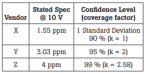
As Figure 1 shows, the three calibrators can be expected to have identical performance because their confidence intervals apply to different areas under the same curve for the normal distribution of uncertainty.

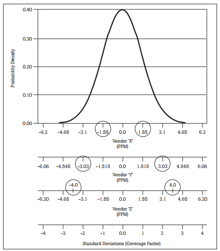
Figure 1. Same performance, different specifications.

In the example above, Vendor X, with a confidence level of 90 %, or 1 standard deviation, is acknowledging that approximately 10% of the calibrators it produces may not meet the 10 V specification of 1.55 ppm.

Fluke uses a 99 % confidence level for its specifications for calibrators and standards. As a buyer, one should be alert to the issues surrounding the confidence level for a specification and should ask the vendor to clarify the confidence level when there is doubt as to what it is.

Beware of the word “accuracy”

Typically, the number on the cover of a data sheet or brochure will read “Accuracy to xx ppm.” What it really means is “xx ppm uncertainty.” This is the result of imprecise language: substituting “accuracy” when “uncertainty” is intended. One also needs to be aware that a specification such as this is often over the shortest time interval, the smallest temperature span, and is sometimes a relative specification.

Components of a specification

Determining an instrument’s true specifications requires that all important specifications be combined. For this discussion, the uncertainty terms comprising calibrator specifications are divided into three groups: baseline, modifiers, and qualifiers.

• Baseline specifications describe the basic performance of the instrument.
• Modifiers change the baseline specifications, usually to allow for the effects of environmental conditions.
• Qualifiers usually define operating limits, operating characteristics, and compliance with industrial or military standards.

The following paragraphs describe each in detail.

Baseline specifications

Baseline specifications consist of three components. They are listed here along with the name used to represent them in this application note:

• output
• scale
• floor

The general form for a baseline specification can be expressed as: ± (output + scale + floor)

Where:

output = percent or parts per million (ppm) of the output or setting

scale = percent or ppm of the range, or full-scale value of the range, from which the output is supplied (some times given as a fixed value in units or as digits)

floor = a fixed value in units

One or more of these terms will be present in the specification, though not all specifications will include all the terms.

The output term of the baseline specification is often quoted casually to describe the instrument’s capabilities. But this output uncertainty term alone should not be used to technically evaluate the unit’s actual performance. The other two terms can make a significant contribution to the total uncertainty. The following discussion shows how the three terms are combined. Refer to the calibrator specification graph in Figure 2.

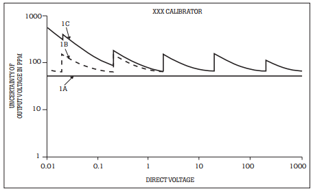
Figure 2. Baseline specifications.

The output term

Line 1 A is output—the uncertainty of the basic output signal. This 50 ppm uncertainty term shows up as a horizontal line. It is a constant percentage of output for all settings of the calibrator.

The scale term

Line 1B in Figure 2 includes scale. The scale term is the uncertainty associated with the output range. Whether specified as a percentage of full scale, or as a percentage of range in units or digits, scale describes the fixed uncertainty for a specific range. This means that although the magnitude of the scale term is the same for all outputs across the range, the effect it has at the low end of the range is greater. At the low end it represents a larger portion of the output than it does at full scale.

Note that Line 1B takes on a saw-tooth form. The peaks of the sawtooth are where the next-highest range is selected. This profile is caused by scale being a larger percentage of a fractional scale output. For example, on the 20 V range, the 10 ppm uncertainty of the fullscale 20 V value is 200 mV. This uncertainty applies to any output on the 20 V range whether it is 3.0 V or 19.93 V.

Two steps are performed here to translate the scale uncertainty term to a specific percentage of any given output value. First, scale was converted to microvolts, using the full-scale output level. This magnitude was then converted to ppm at each specific output value.

The floor term

In addition to a calibrator’s uncertainty relative to its output and scale, there can be additional uncertainty of a fixed magnitude. This is typically an offset, but can also include noise. This added uncertainty is called the floor, and, for any given range, it is constant across that entire range. For example, often a calibrator specification will include a description such as, “with a floor of 5 mV.” This is the floor specification. Because this constant error is a greater percentage of small outputs than of large outputs, it becomes more important as the magnitude of the output decreases.

Line 1C in Figure 2 includes floor. This term can vary by range or can be a constant across all ranges. Floor uncertainty is similar to scale and may be combined with the scale term for simplicity. Adding this term to the baseline uncertainty plot shown in Figure 2 raises the curve even farther, particularly on the lower end: the constant voltage uncertainty is a large percentage of the total output for smaller voltages. In a more extreme example, a 5 µV floor amounts to an additional 5 ppm uncertainty at 1 V, whereas 5 µV is only an additional 0.025 ppm uncertainty at 200 V output.

The true baseline calculation

Comparing Line 1C with Line 1A shows that the total baseline uncertainty specification is quite different from the basic output uncertainty specification. Yet the total uncertainty specification must be used in determining whether the calibrator will actually fill your needs. This total uncertainty specification must support your application or workload even at the low end of each range.

The comparison of Line 1A to 1C is not as bad as a quick reading of this discussion may first cause one to believe. This is because we are using voltmeters and calibrators as examples. The sawtooth calibration specification in Line 1C is different from 1A, but a voltmeter behaves in the same way and its specifications would reveal much the same pattern so the calibrator could be used to support it at nearly the same Test Uncertainty Ratio (TUR) for all values.

The next questions to be answered are: What do the numbers in the baseline specification include? Under what conditions do these specifications apply? This is where the modifier and qualifier specifications are brought in.

Modifier specifications

Modifier specifications change the baseline specifications. Most manufacturers include modifiers as part of the baseline specification so that one doesn’t need to calculate these, though not all do this. The most important modifiers include instrument stability over time, the time interval for which the specifications are valid, and changes in specifications with changes in temperature (the ambient temperature of the instrument’s operating environment rather than its internal temperature). Other secondary specifications include the effect of inductive and capacitive loading, no load versus full load operation, and any changes due to changes in line power.

Modifier specifications are important because the application may require particular aspects of performance to be detailed. Figure 3 shows the plot of the secondary specifications for the direct voltage output of a calibrator.

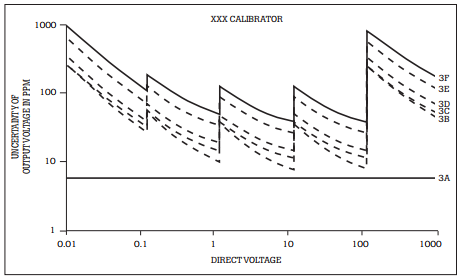
Figure 3. Secondary specifications.

Line 3A is a plot of the basic output uncertainty stated in the manufacturer’s data sheet. As previously mentioned, this is the number that is often casually quoted to describe the calibrator’s performance. Line 3B is the total baseline uncertainty (output + scale + floor) for 24 hours, at an operating temperature of 23 ± 2 °C at no load. Now the effects of the modifier specifications will be added.

The time term

Specifications usually include a specific time period during which the instrument can be expected to perform as specified. This is the calibration interval, or the measure of an instru-ment’s ability to remain within its stated specification for a certain length of time.

Limiting this time period or calibration interval is necessary to account for the drift rate inherent in an instrument’s analog circuitry. Time periods of 30, 90, 180, and 360 days are common and practical. Any calibrator can be specified to super-high performance levels at the time of calibration. Unfortunately, such levels are good for only the first few minutes following calibration. Any instrument may drift beyond realistic performance levels. If the specifications for an instrument do not state the time interval over which they are valid, a stability factor corresponding to the desired time interval will have to be added.

Some vendors specify the time term as a function of the square root of the years. Recent work at Fluke indicates that the square root of the years method of specifying an instrument may not be appropriate. Fluke experiments indicate that the long term drift of well-aged voltage and resistance standards is nearly linear with time. However there can be short term excursions from a linear regression due to the superposition of low frequency noise on the basic drift. For short periods of time, the accumulated linear drift is small in comparison to the noise excursions, so a short term, e.g. 90 days, uncertainty specification predominantly reflects the uncertainty due to low frequency noise. However, the long term, e.g. 1 year specification, includes the effects of accumulated linear drift.

The calculation of the time term due to calibration interval is based on the root/years’ square rule. Simplified, it takes the form: rys = y√i

Where:

rys = root/year specification

y = 1 year specification

i = desired calibration interval in years

As the equation suggests, an instrument’s 1 year specification is published by its vendor. Specifications for other intervals are user computed by multiplying the 1 year specifications by the square root of the number of years for which they are intended to apply. For example, a period of 90 days is about 0.25 years so the square root of 0.25 (0.5) is used to multiply the 1 year specifications to obtain the 90 day specifications.

While the specifications for Fluke calibrators include variation in performance due to the passage of time, other calibrators may not be specified in the same manner. In this case the specification for their stability with time must be added as line 3C in Figure 3.

The temperature term

Equally important is performance over the specified temperature range. This range is necessary to account for the thermal coefficients in the instrument’s analog circuitry. The most common ranges are centered about room temperature, 23 ± 5 °C This range reflects realistic operating conditions. It should be remembered that temperature bounds must apply for the whole calibration interval. Thus a temperature range specification of 23 ± 1 °C presumes very strict longterm control of the operating environment.

Outside the specified range, a temperature coefficient (TC) is used to describe the degradation of the uncertainty specification. The temperature coefficient is an error value which must be added to an instrument’s baseline specification if it is being used outside of its nominal temperature range. Look at the temperature coefficient graph shown in Figure 4.

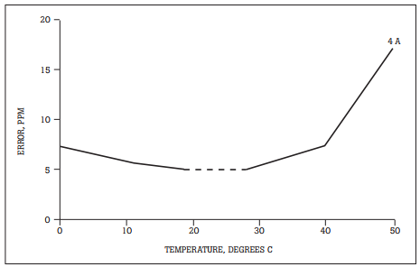
Figure 4. Uncertainty due to temperature

The x-axis is temperature and the y-axis is uncertainty. The dashed portion of Line 4 A shows the specified uncertainty for a 23 ± 5 °C temperature range common on most Fluke calibrators. Within the span of the dashed line, the uncertainty is within the specifications of 5 ppm. This is in line with a baseline specification of “± 5 ppm when used at 23 ± 5 °C.” This is an absolute range of 18 °C to 28 °C Beyond this range, the instrument’s performance degrades as shown by the solid TC line. TC will usually be given in a specification footnote, and will take the form: TC = x ppm ⁄ °C where x is the amount that the performance degrades per change in degree beyond the base range specification. To calculate the uncertainty due to temperatures outside of the given specification, the temperature modifier, tmod, is needed.

The formula is: tmod = |TC x ∆t|

Where:

∆t = operating temperature minus the temperature range limit

t = the proposed operating temperature

range limt = the range limit that t limit is beyond

If one wishes to use a calibrator in an ambient temperature outside of its specified range, the effects of TC must be added to the baseline uncertainty specification when calculating the total uncertainty. The tmod term is used to calculate the total specification using the general formula: total spec = (basic uncertainty at a specific temp. range)+tmod.

For example, suppose we have a calibrator whose rated uncertainty is 8 ppm @ 23 ± 2 °C. Its TC is 3 ppm/C°. To calculate the uncertainty of the calibrator for operation at 30 °C:

t = 30

range limit = 23+2 = 25

tmod = 3 ppm|30-25| = 3 ppm|5| = 15 ppm

total spec = 8 ppm + 15 ppm = 23 ppm

As can be seen, the specification changes dramatically when the effects of performance due to temperature are considered.

Knowing how to calculate tmod will be necessary when comparing two instruments that are specified for different temperature ranges. For example, Fluke specifies most of its calibrators with a range of 23 ± 5 °C However, another manufacturer may specify a calibrator at 23 ± 1 °C To truly compare the two calibrators, one needs to put them in the same terms (23 ± 5 °C) using the preceding calculation.

The most modern calibrators and instruments are specified to operate in wider temperature ranges. This is because calibration instruments are no longer used only in the closelycontrolled laboratory. Calibration on the production floor demands greater temperature flexibility. The preceding equation was used to characterize the degradation in performance that occurs when the calibrator is operated outside the 23 ± 2 °C temperature range restriction on the data sheet. The result is Line 3D in Figure 3.

Power line and output load terms

In the modifier example, another footnote lists an uncertainty modifier for an assumed line voltage variation of ± 10 % of rated uncertainty. Adding this results in Line 3E in Figure 3. Finally, one last footnote covers an uncertainty modifier for load regulation. This term must be included in the total uncertainty calculation because loading the calibrator is necessary for use. Adding the uncertainty for 0 % to 100 % load to Line 3E yields Line 3F in Figure 3.

The modified baseline specification

Notice how the total uncertainty changes when adding terms of calibration interval, temperature, and line and load regulation. Comparing Line 3A with Line 3F reveals that the actual uncertainty under operating conditions is 10 to 100 ppm worse than the specified 6 ppm. One must carefully review all of the specifications to assess whether an instrument will really meet the requirements. Again, the instrument must satisfy the application even at the low end of each range where the specification deteriorates.

Qualifier specifications

The uncertainty terms that can be considered qualifier specifications rarely affect the general specifications or analog performance, but they may be important to the application. These are performance limits and operating characteristics that include emi effects, humidity, and altitude. FCC and military standards such as MIL-T-28800C cover emi emissions and some aspects of emi susceptibility, but there may still be complications. For example, emi from a nearby crt could adversely affect a precision instrument lacking adequate shielding. Compliance with safety standards such as UL, CSA, VDE, and IEC may also be important in your application. These must be kept in mind when comparing instruments.

Relative versus total specifications

Uncertainty specifications must also be evaluated as relative or total. Relative uncertainty does not include the additional uncertainty of the reference standards used to calibrate the instrument. For example, when a calibrator’s uncertainty is specified as relative to calibration standards, this covers only the uncertainty in the calibrator. This is an incomplete statement regarding the instrument’s total uncertainty. Total uncertainty includes all uncertainties in the traceability chain: the relative uncertainty of the unit, plus the uncertainty of the equipment used to calibrate it. This is the true specification of available instrument performance.

A standards laboratory can provide the uncertainties in their calibration standards. These uncertainties must be combined with the specifications relative to calibration standards to determine the performance which is actually achieved. In general, Fluke’s practice is to state the more useful total specification, which assumes calibration was in accordance with the instrument operator’s manual.

The units of the specification

Using different units also adds confusion. Output, scale, and range can be quoted in percentages or parts per million. Scale, range, and floor can also appear as digits or volts. It may be necessary to interpolate between units. The general formulas to convert from % to ppm and back are:

ppm = % x 104

% = ppm ⁄ 104

Table 2 shows the relationship of some commonly-used ppm and % values.

Table 2. The relationship of PPM to percent

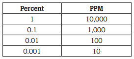
As is shown later, a good way to compare specifications for calibrators and DMMs is by converting all of the % and ppm terms to microvolts first. The formulas are:

specmv = specppm (output in volts ⁄ 10-6)

and

specmv = spec% (output in volts ⁄ 10-4)

Comparing specifications: A detailed example

Now it’s time to compare the specifications for two different models of calibrator. Tables 3 and 4 depict two typical specification tables found in the literature for modern calibrators. Baseline specifications for Calibrator B appear to be four times better than for Calibrator A but are they really?

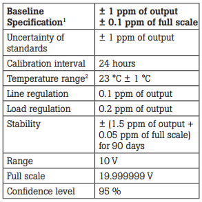
Table 3. Calibrator A

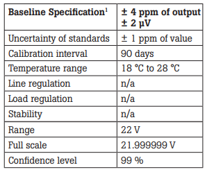
1Baseline specifications include the uncertainty of standards, temperature coefficient for the temperature range, the effects of line and load regulation as well as stability during the calibration interval.

Table 4. Calibrator B

1Relative to calibration standards

2TC = 0.4 ppm⁄°C

Comparing these two calibrators requires:

• Identifying the specifications that need to be converted
• Converting applicable specifications to microvolts
• Adding the microvolt values
• Adjusting uncertainty for stated confidence interval

Take a look at the process of getting the results.

Identifying the items to be converted

List all of the relevant specifications for both calibrators that apply to the situation at hand. Here, it is the comparison of the total uncertainty of both calibrators at an output of 19.99999 V. Table 5 is a result of the listing. For calibrator A, the baseline specification and the range floor are the only items to be converted to microvolts. All of the other baseline modifiers are included in the baseline specification.

Calibrator B needs several more conversions, because all of its baseline components and modifier specifications are listed individually. Along with the baseline specification and range floor, the standard uncertainty, calibration interval, line regulation, load regulation, and stability must all be converted to the appropriate terms. Calibrator B has a maximum range of 19.99999 V. This is effectively 20 V, so one would use that for the output value.

Also, although both calibrators have footnotes stating a TC of 0.4 ppm/°C, Calibrator A is exempt from including any temperature modifier because its specifications encompass the widest range. Calibrator B’s specification will have to be modified for TC. See Table 5.

Converting the specifications

Convert the baseline specifications for both calibrators to microvolts, then add in the specifications that aren’t included in the baseline specifications. This will give the total specified uncertainty for both calibrators at 20 V The results of the conversion and calculation are shown in Table 6.

For the benefit of the doubt, this test assumes a high-impedance DMM load. Even though Calibrator B’s load uncertainty is 0.2 ppm of output, its load modifier is 0.0 mV. Low impedance loads could cause this entry to rise to 40 mV at full load current.

Applying the confidence interval

In this adjustment, the ratio of the desired to specified confidence interval is used to multiply the total specified uncertainty of each calibrator. This operation yields specifications that have the same confidence level. The ratios of the confidence intervals are used as multipliers because it is assumed that the specifications reflect a normal distribution of uncertainty. In other instances, the t factor is used as a multiplier.

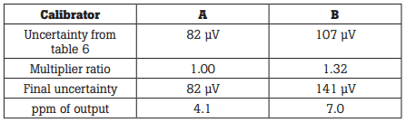
For these purposes, it is enough to know the following: 99 % confidence level = 2.58 confidence interval 95 % confidence level = 1.96 confidence interval.

From this, one can find that the multiplier ratios are 2.58/2.58 = 1.00 for Calibrator A, and 2.58/1.96 = 1.32 for Calibrator B.

Now each total specified uncertainty from the preceding Table 6 is multiplied by the multiplier ratios. Using the ratio of desired to specified interval, the specifications for Calibrators A and B are adjusted for the desired (higher) confidence level, 99 %. The results are shown in Table 7.

In the original specification, Calibrator B appeared to be four times as accurate as Calibrator A. But with all of the additions and corrections needed to interpret Calibrator B’s specifications, it turns out that Calibrator B is about 72 % less accurate than Calibrator A. That is, its uncertainty is 72 % greater under identical conditions.

Table 5. Pre-conversion tabulation

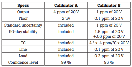
Table 6. Microvolt equivalents and totals

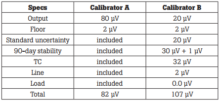
Table 7. Results of comparison

Other considerations

Uncertainty specifications are an important part of determining whether or not a particular calibrator will satisfy the need. There are, however, many other factors that determine which instrument is best suited for an application. Some of these are listed as follows.

The workload: Remember that the instrument’s specification must match the workload requirements. There is a tendency for manufacturers to engage in a numbers race, with each new instrument having more and more impressive specifications, although often this has little bearing on true workload coverage.

Support standards: The support standards will typically be three to ten times more accurate than the instruments supported. This is known as the test uncertainty ratio (TUR). Specialized instruments or those that require exotic support equipment on an infrequent basis may best be served by an outside service bureau.

Manufacturer support: One should also consider the level of manufacturer support. Can the manufacturer provide support as calibration needs grow and vary? Do they have in-house experts who can assist with technical issues? Are training programs available? Are service facilities conveniently located? Do they have an adequate line of support products and accessories?

Reliability: Reliability is another important consideration in how useful an instrument will be. Precision electronic instruments can have a seemingly high failure rate. Any condition that causes the instrument to fall outside of its extremely tight tolerance constitutes a failure. One should ask for a Mean Time To Fail rate (MTTF) to determine when the first failure might occur. Failures upon delivery usually make this interval shorter than the Mean Time Between Failure rate (MTBF). Whichever is quoted, consider whether the number is based on actual field experience or just calculated projections.

Service philosophy: When an instrument does fail, the manufacturer’s approach to service becomes very important. A responsive service organization is essential to getting equipment back in action fast. Issues to consider include service center locations and one’s proximity to them, stocking levels for spare parts and subassemblies, availability of service manuals, and service training for one’s own technicians, all of which go into determining how soon equipment can be returned to service.

Reputation: Finally, the manufacturer’s reputation should be assessed. Overall, how credible are its claims with respect to performance, reliability, and service? Will the company still be around five years from now? All of these issues define the true cost of owning and using a calibrator.

Need any help or have any requirements? Speak to one of our technical sales engineers:

This application note has been adapted from “Chapter 31: Instrument Specifications,” in Calibration: Philosophy in Practice, Second Edition.